


I decided to create a series of two articles dedicated to the Finite Element Method (FEM) theory. I’m writing this because I’ve been receiving many questions on the topic, and it also came up repeatedly in a survey I ran a few months ago, where I asked what topics you’d like me to cover.
Two subjects stood out: how the global stiffness matrix is assembled, and how the solver computes the linear equations.
So I’m kicking off this series on FEM theory, split into two parts:
FEM Theory Part #1: How Is the Global Stiffness Matrix Assembled?
FEM Theory Part #2: How Does Your FEA Solver Compute the Linear Problem Without Inverting the Stiffness Matrix?
The Equilibrium Equation
With the finite element method, a continuous system described by differential equations is represented by a discrete system called the mesh. The discrete system is a collection of elements connected at nodes. This process of discretization makes it possible to transform a real problem governed by partial differential equations, which cannot be solved by a computer, into a structural model governed by matrix equations that can be solved by a computer.
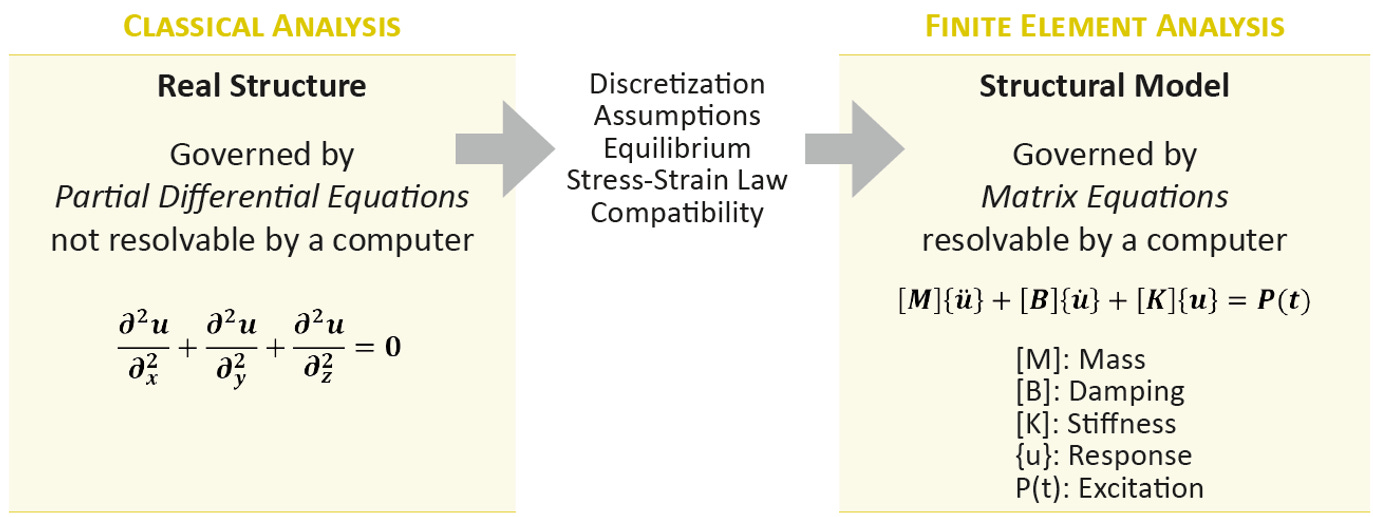
A structural problem with an infinite number of degrees of freedom is converted into a problem with a finite number of degrees of freedom. When the nodes are displaced, the elements have an elastic response within their domain, providing a representation of the elastic properties of the complete system.
For continuum mechanics problems, the unknown quantities of the mathematical model are the nodal displacements.
The finite element method is based on the following matrix equation, known as the General Equilibrium Equation of Mechanics, which defines the state of equilibrium of forces acting on a structure:
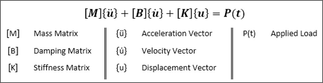
Since this article focuses on stiffness matrix assembly, we’ll assume the problem involves no dynamic effects. In other words, mass and damping are negligible, and the problem reduces to a static one. As a result, the general equilibrium equation above simplifies to:
[K]{u} = {P}
In this equation, the unknown is the displacement vector {u}, and we'll see in Part #2 how the solver computes the solution. The vector {P} represents the applied loads acting on the mechanical system, defined from all load types applied at the nodes (forces, pressure, enforced displacements, thermal effects, etc.). The stiffness matrix [K] is known and corresponds to the global stiffness of the mechanical system. This stiffness matrix is calculated at each node for the collection of degrees of freedom associated with each node, which themselves depend on the element formulation selected by the modeler.
Element & Global Stiffness Matrix
The chart below summarizes the process for generating the global stiffness matrix for a given problem. The first three stages fall under the analyst’s responsibility: creating the mesh and applying the geometric and material properties to the elements. The solver then takes over, with the computation of the stiffness matrices being one of its first tasks.
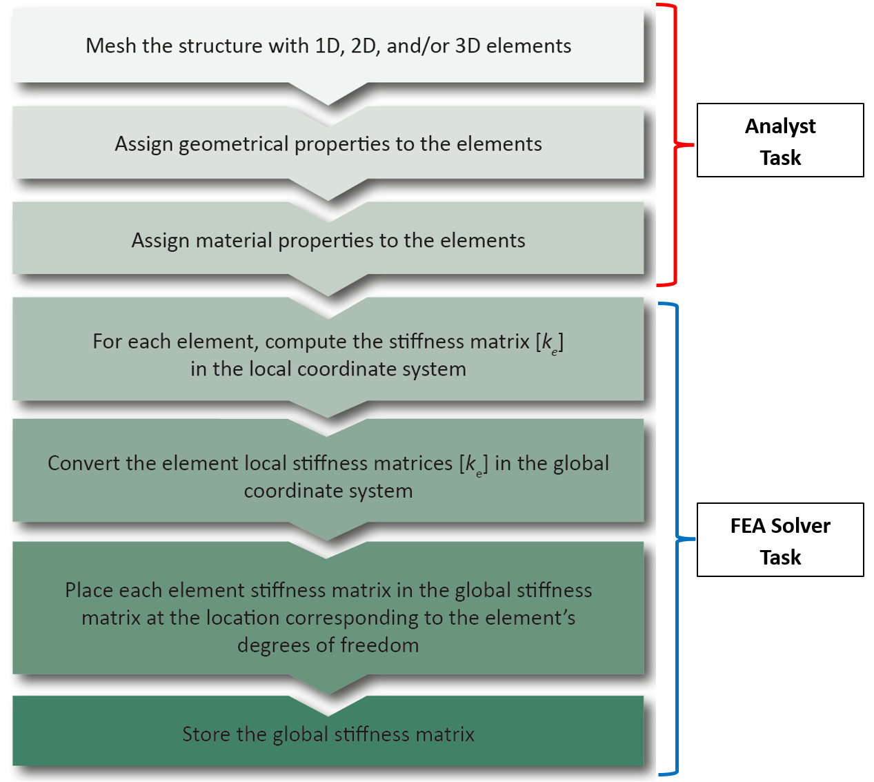
For each element composing the structural mesh, the stiffness matrix is computed in the element’s local axis and then transformed into a global coordinate system common to all elements.
The stiffness matrix is an inherent property of the structure: it is square and symmetric and includes only positive diagonal terms. Once the element stiffness matrices are calculated, they are assembled into a single global stiffness matrix based on how the elements are connected.
The stiffness at a given node is obtained by summing the stiffness contributions of all elements connected to that node. Assembling the global stiffness matrix therefore consists of placing each element’s degrees of freedom in their proper position within the global stiffness matrix of the whole structure (I’ll illustrate this later with an example).
Which Parameters Influence the Element Stiffness Matrix?
The stiffness matrix is affected by several parameter:
The type of elements selected by the analyst and their formulations
The material properties assigned to the elements
The mesh quality
The boundary conditions
The connections between elements
Keep in mind that these parameters, as defined by the analyst, are critically important, because the stiffness matrix computation allows us to answer several key questions:
Where is the structure stiff and where is it flexible?
How are the loads distributed among the different components of the structure?
Which parts move when external loads are applied on the structure and how much do they move?
The Generic Form of the Element Stiffness Matrix
In Chapter 5 of my book, Practical Finite Element Analysis for Mechanical Engineers, I present the fundamentals of FEM theory, including how element stiffness matrices are computed for 1D, 2D, and 3D elements. You can also find these details in my article “The Finite Element Theory in Depth” available on the FEA Academy website.
For this article, however, I’ll simply remind you that the following equation, derived from the virtual work principle, allows us to compute the element stiffness matrix for any element used in a finite element model:

where:
[B] is the Strain-Displacement Matrix. The form of [B] depends on the shape function used to describe the displacement field in the element.
[D] is the Constitutive matrix (related to the material data)
Global Stiffness Matrix Assembly
To explain how the global stiffness matrix is assembled by the solver, I am going to take a simple example. Let’s consider a simple rectangle plate discretized using four constant strain triangular (CST) elements, as shown on the figure below:
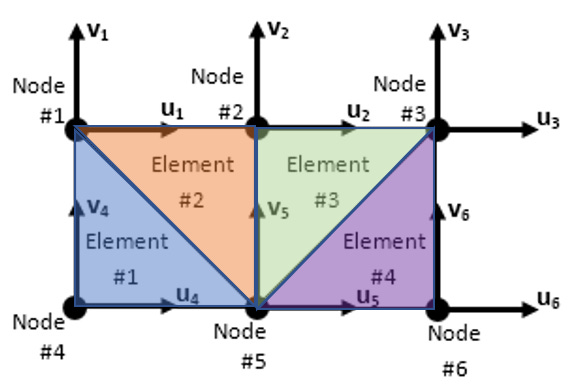
Six nodes are involved in this discretization.
Each CST element has two degrees of freedom at each node, so the total number of degrees of freedom for the plate is 6 x 2 = 12.
Then, the stiffness matrix for the plate meshed with four CST elements will have a size of 12 x 12.
As mentioned at the beginning of this article, the assembly of elements consists of placing each elemental matrix in the appropriate position within the global matrix, based on the degrees of freedom associated with each element.
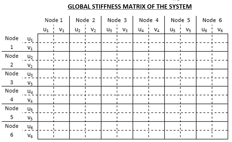
The element stiffness matrices for each CST elements are computed numerically by the FE solvers, using the geometrical and material data assigned to each element.
Let’s see what the solver is doing element by element.
Element #1
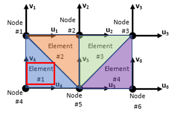
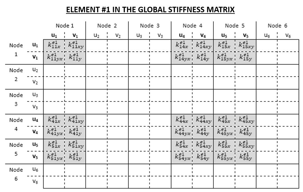
Element #1 is connected at nodes #1, #4, and #5. The degrees of freedom involved in constructing the stiffness matrix for element #1 are: (u1, v1), (u4, v4), and (u5, v5). So, we know that the stiffness matrix for element #1 is written as (note that the nodes are considered anti-clock wise):
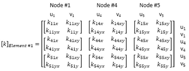
So, for the element #1, the global stiffness matrix is populated as:
Element #2
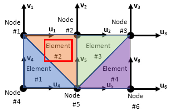
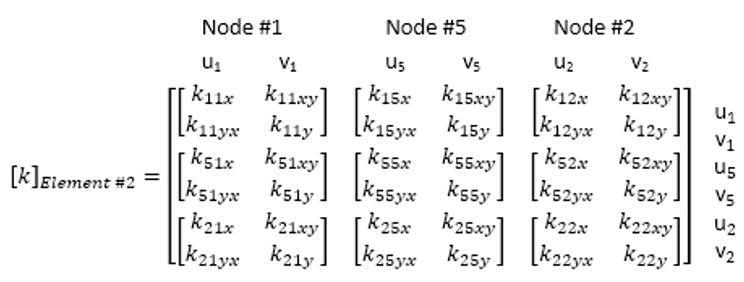
Element #2 is connected at nodes #1, #2, and #5. The degrees of freedom involved in constructing the stiffness matrix for element #2 are: (u1, v1), (u2, v2), and (u5, v5). So, we know that the stiffness matrix for element #2 is written as (note that the nodes are considered anti-clock wise):
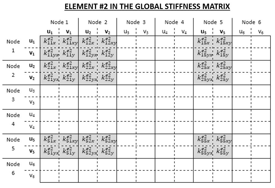
So, for the element #2, the global stiffness matrix is populated as:
Element #3
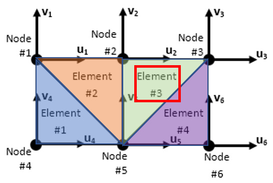
Element #3 is connected at nodes #2, #3, and #5. The degrees of freedom involved in constructing the stiffness matrix for element #3 are: (u2, v2), (u3, v3), and (u5, v5). So, we know that the stiffness matrix for element #3 is written as (note that the nodes are considered anti-clock wise):
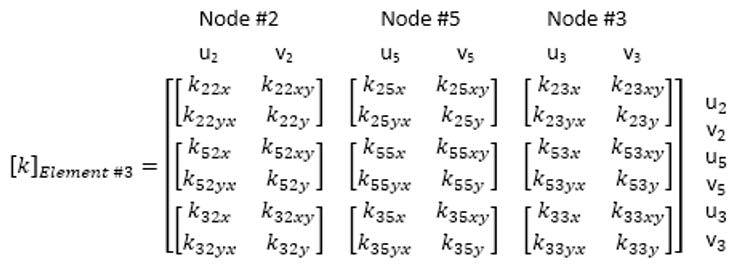
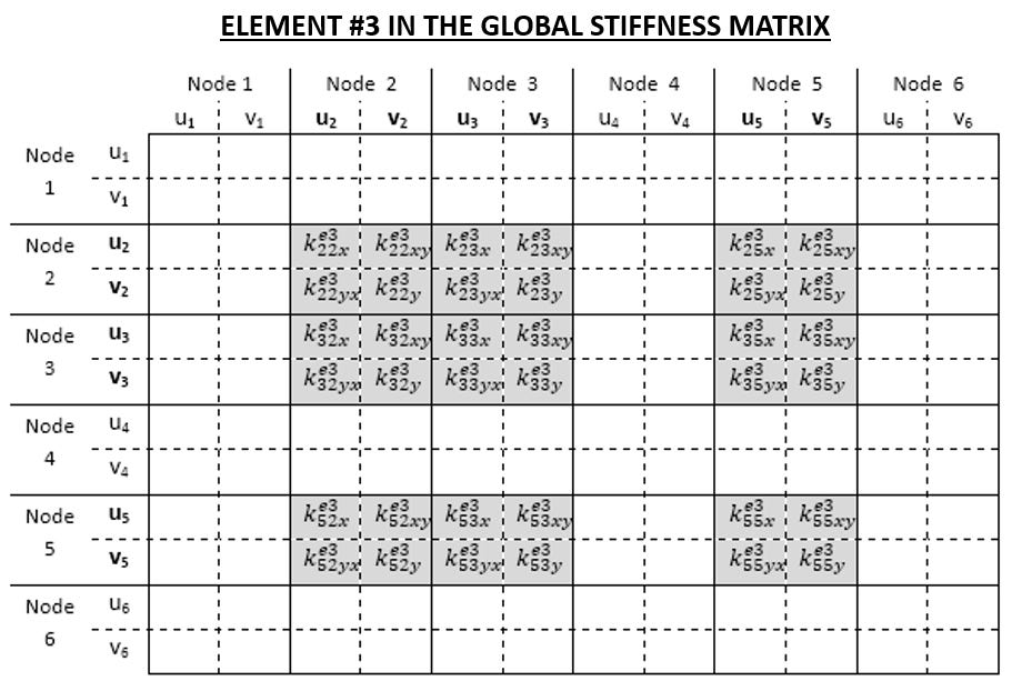
So, for the element #3, the global stiffness matrix is populated as:
Element #4
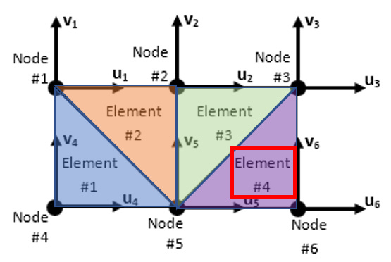
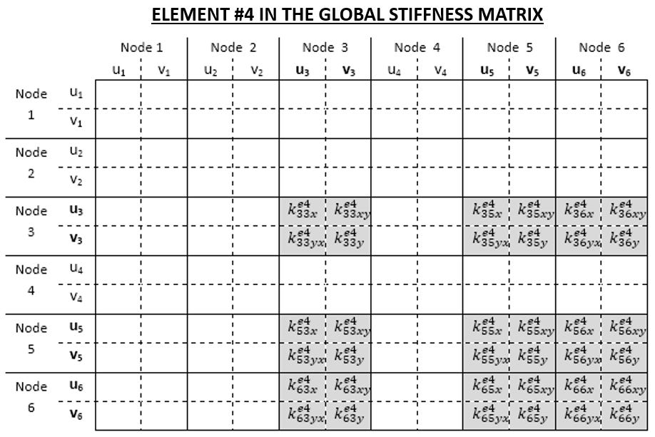
Finally, the element #4 is connected at nodes #3, #5, and #6. The degrees of freedom involved in constructing the stiffness matrix for element #4 are: (u3, v3), (u5, v5), and (u6, v6). So, we know that the stiffness matrix for element #4 is written as (note that the nodes are considered anti-clock wise):
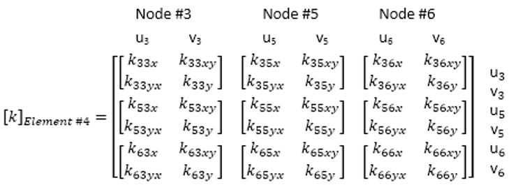
So, for the element #4, the global stiffness matrix is populated as:
Assembly
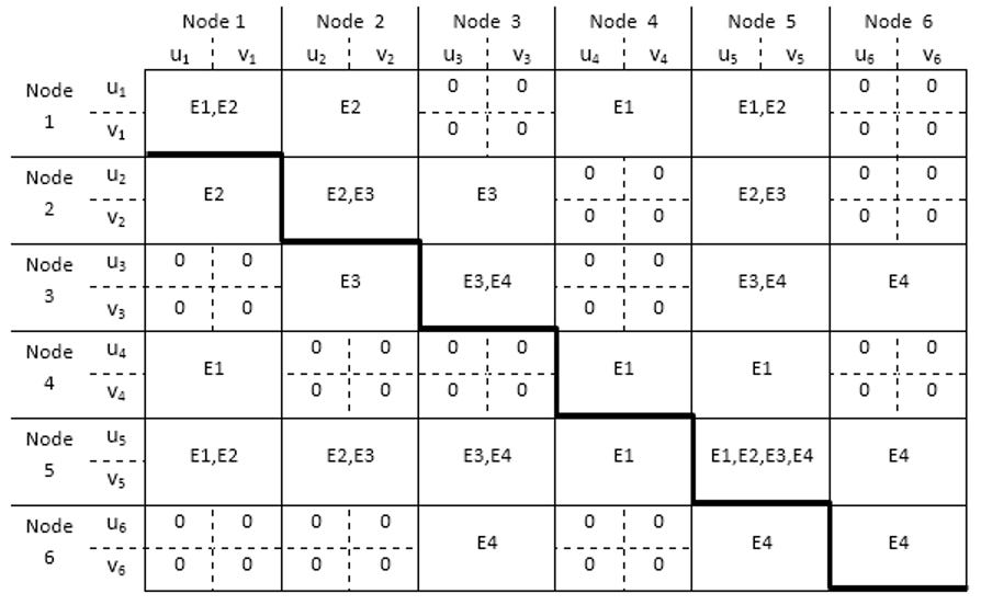
The figure below shows the assembly of the elements with their associated degrees of freedom (ui,vi) for i = 1 to 6.
Half of the positions in the matrix have null values.
The stiffness matrix is symmetric.
Only the upper portion of the stiffness matrix must be computed and stored to perform the structural analysis.
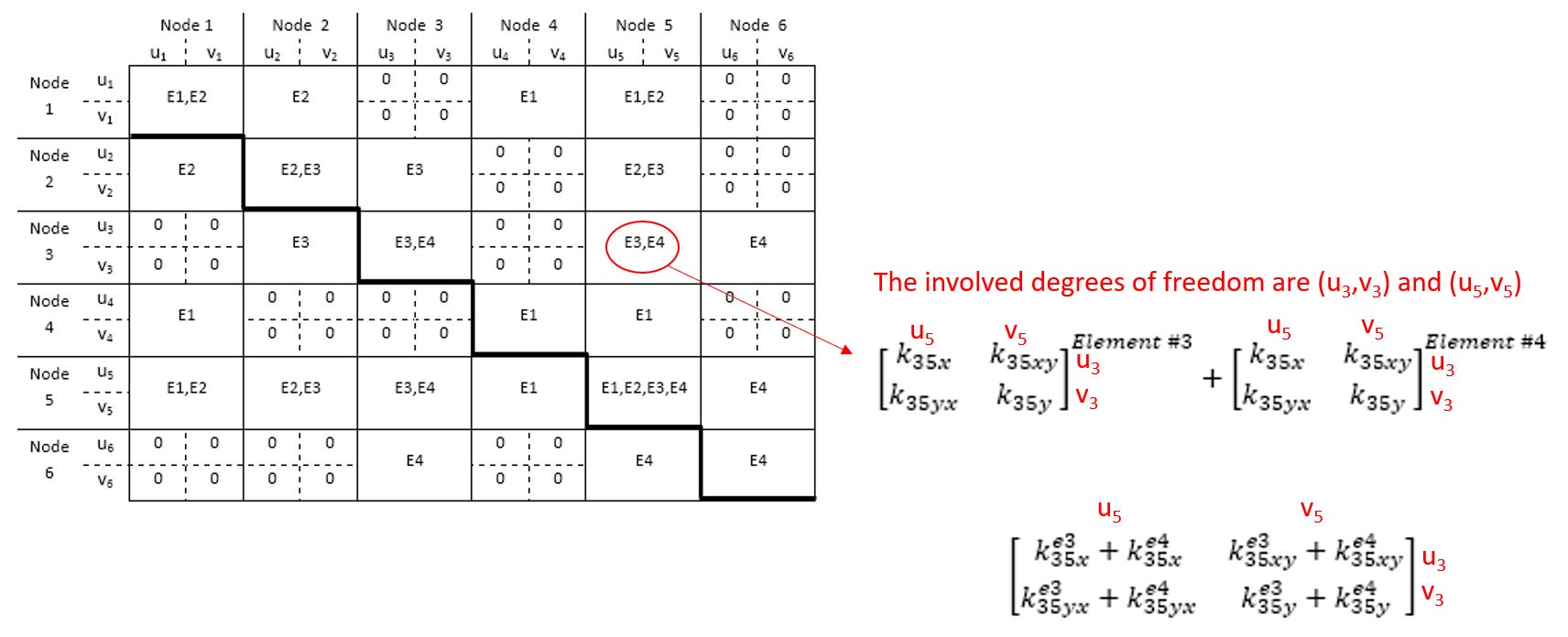
The global structure stiffness matrix [K] for the rectangle plate meshed with four constant strain triangular elements is obtained using the direct stiffness method:

Now you know how your FEA solver assembles the complete stiffness matrix for your finite element model. In the second part of this series on FEM theory, we’ll look at how your FEA solver computes the linear problem without inverting the stiffness matrix.
Extremely happy having found on Substack a newsletter like yours. I am new here and this is the niche topics I was looking for.
About the article itself I must admit that assembling the stiffness matrix for MDOF systems is so satisfying in my opinion. Eventually after assembling you may end up with quite big matrices out there :)
Structural integrity in security operations relies on understanding how individual components contribute to the total defense posture. When you map these dependencies, you move past simple compliance and start building actual visibility into your environment. Most teams treat the assembly of their security stack as a box-ticking exercise to satisfy auditors. True visibility requires accepting that the cost of ignorance always exceeds the cost of implementation. By choosing to see the gaps rather than hiding them behind a facade of checkboxes, you transform your architecture into a genuine asset. This is how you stop paying for the illusion of safety and start investing in real detection.
https://cyrilsimonnet.substack.com/p/the-cheapest-way-to-comply-is-to?utm_source=substor&utm_medium=substack&utm_campaign=comment