



In this second part of the series on FEM theory, I want to cover the solving aspect. If you missed the first part, it covered how the global stiffness matrix is assembled, illustrated for a simple flat plate discretized with four triangular CST elements. Here is the link to the first part: FEM Theory Part #1: How the Global Stiffness Matrix is Assembled?
In this second part of the series, we will look at how the solver computes the equation [K]{u} = {P}, which is the governing equation for a mechanical static problem.
Contrary to what you might expect, even though the unknown in this equation is the displacement vector {u}, and the stiffness matrix [K] and load vector {P} are known and defined by the analyst, the solver does not invert the stiffness matrix to compute the solution as {u} = [K]-1{P}. The reason is efficiency: inverting a matrix that describes a problem with millions of degrees of freedom is computationally expensive and impractical.
The method used to solve the equation [K]{u} = {P} is known as the direct method based on LDLᵀ decomposition.
If like me you are curious about history, the method is attributed to André-Louis Cholesky, a French military officer and mathematician, who developed it around 1910 for geodetic survey calculations. He never published it himself; it appeared posthumously in 1924 (he died in World War I in 1918), credited to him by a colleague, Commandant Benoit. Alan Turing later made a separate contribution. In his 1948 paper “Rounding-Off Errors in Matrix Processes,” he gave the first elegant treatment of Gaussian elimination as a triangular decomposition (LU, and by extension LDLᵀ), along with an error analysis that became foundational to modern numerical linear algebra. Cholesky discovered the algorithm; Turing gave the framework it’s now presented within.
Three Steps
With the direct method, the equilibrium equation {P} = [K]{u} is solved for unknown displacements {u}, without inverting [K]. LDLT decomposition, the matrix form of Gaussian elimination, is an efficient and accurate method, comprised of three steps:
Step #1: Factorization, using the Cholesky decomposition
Step #2: Forward Substitution
Step #3: Backward Substitution
Let’s these three steps in detail.
Step 1: Factorization
Using the Cholesky decomposition, the stiffness matrix [K] is replaced by the product of three matrices: [L], [D] and [L]T:
[K] = [L].[D].[L]T
[L] is the unit lower triangular matrix
[D] is the diagonal matrix
[L]T is the unit upper triangular matrix
We can illustrate the factorization for a n x n matrix as follows:
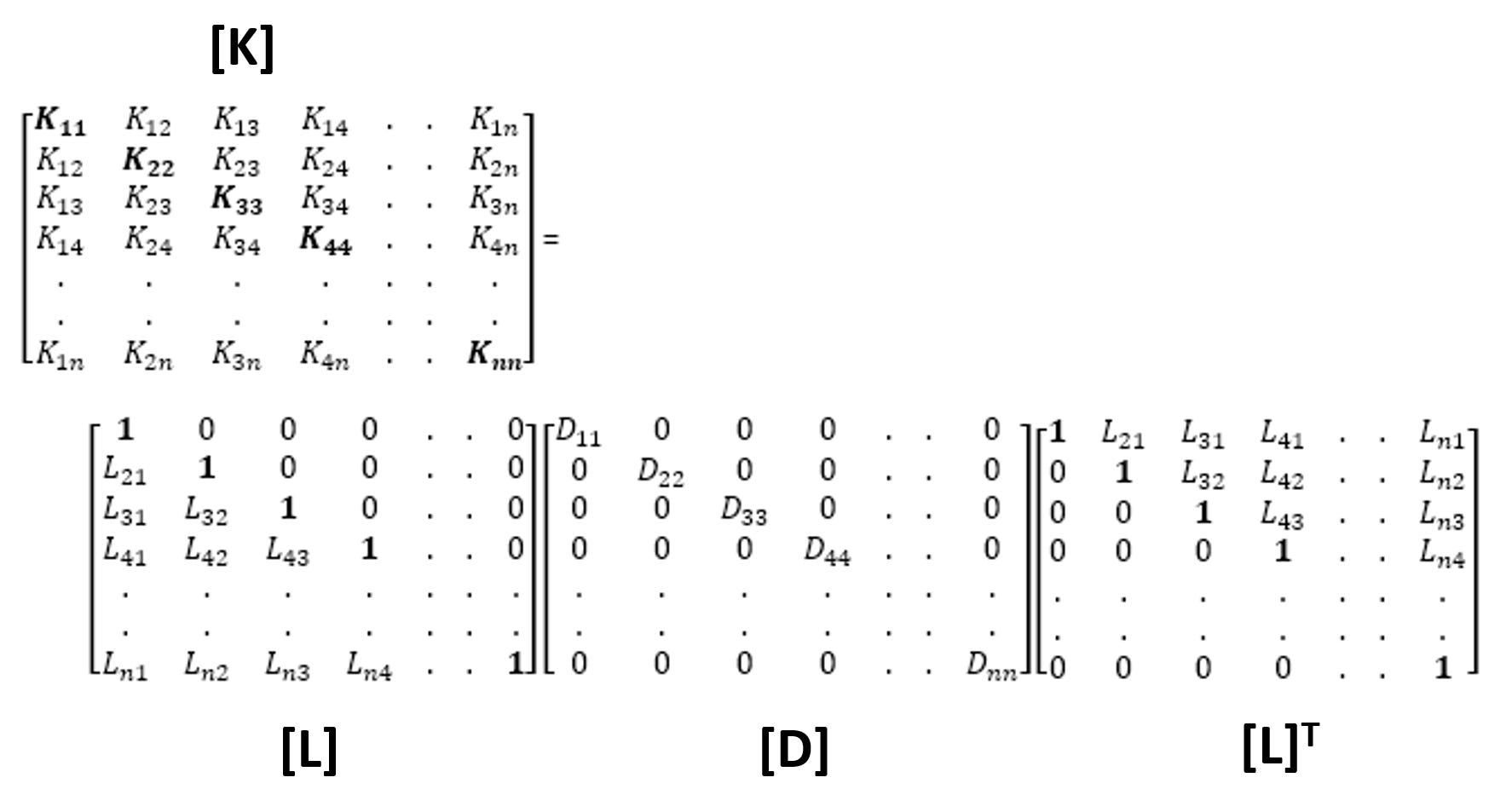
The decomposition results in the stiffness matrix [K] being separated into the product of three simple matrices [L], [D] and [L]T.
The decomposition process consists of finding the factors of [D] and [L]. To achieve that, the Cholesky method is used. Indeed, this method is very efficient in terms of memory storage capacity, computational cost, and speed. The Cholesky decomposition factors are computed as:

For i > j

Cholesky decomposition is implemented as follows:
The subscript i is the row index, and the subscript j is the column index.
Decomposition is computed column by column.
Decomposition starts with the evaluation of the diagonal terms in the column, using Equation 1
The other elements are evaluated row by row, using Equation 2
Step 2: Forward Substitution
Based on the factorization performed in step 1, the equilibrium equation can be written as:
[P] = [K]{u} = [L].[D].[L]T{u} (Equation 3)
Let’s consider:
{y} = [D].[L]T{u} (Equation 4)
Then, the Equation 3 becomes:
[P] = [L]{y}
where {y} is now the unknown.
We can compute {y}, starting with the first equation in the system [P] = [L] {y}
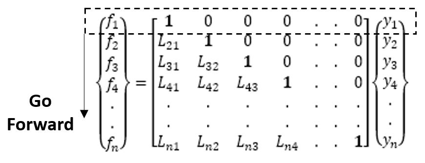
Starting from the first equation: f1 = y1
…and continuing with the next lines, using the results obtained from the previous lines:
f2 = L21.y1 + y2 ⇒ y2 = f2 - L21.y1
f3 = L31.y1 + L32.y2 + y3 ⇒ y3 = f3 - L31.y1 - L32.y2
… and so on. Therefore, the solution for {y} is (for i = 2 to n):

We calculated {y}.
Step 3: Backward Substitution
Now, let’s consider again the equation 4 above:
{y} = [D].[L]T{u}
In this equation {u} is now the unknown.
It can be written as:

Using the results obtained for {y} during the Forward Substitution step, we can solve for {u} starting with the last equation:

For i = n, we have: yn = Dnn.un
un is easily found by:

Then, moving backward {u} is solved by (for i = (n-1) to 1):

We know {u}.
Conclusion
As you can see, we solved the linear static problem without inverting the stiffness matrix, using only additions and multiplications through the Cholesky factors and Forward-Backward Substitution (FBS). This method is highly efficient in terms of computation time and memory usage, which is why all modern FEA solvers use it to perform linear static simulations. So the next time you see the messages “Stiffness Matrix Decomposition Performed” and “FBS Completed” in your log file, you will know exactly what the solver did in the background.
Iterative solvers win because they prioritize operational agility over perfect precision. By avoiding the heavy cost of matrix inversion, engineers keep the feedback loop tight enough to actually respond to changing variables in real time. This same logic applies to how we manage security operations today. When we stop trying to solve for every possible state and instead focus on the most probable paths of compromise, we gain the speed required to stay ahead of an adversary. Security teams that treat their detection logic like a static system eventually break under the weight of their own complexity. Choosing efficiency over absolute certainty allows us to scale defense across borders without getting bogged down by the friction of local constraints.
https://cyrilsimonnet.substack.com/p/the-slowdown-has-a-jurisdiction-the?utm_source=substor&utm_medium=substack&utm_campaign=comment