



In this series
This is Part 1 of a three-part series on eigenvalues and eigenvectors, written for practicing structural and FEA engineers rather than mathematicians. The three parts build on each other:
Part 1: The Mathematical Foundation. What an eigenvalue and an eigenvector actually are, how to compute them by hand, and why engineers keep running into this exact equation.
Part 2: From Linear Algebra to Natural Frequencies and Mode Shapes. The same equation applied to free vibration, with a full worked example.
Part 3: How the Same Eigenvalue Problem Predicts Structural Instability. The same equation again, now applied to buckling under compressive load, with a worked strut example and a certification-margin discussion.
You can read each part on its own, but the payoff of this series is seeing that one piece of linear algebra, learned once in Part 1, quietly drives both your modal results and your buckling results in Parts 2 and 3.
Why a Working Engineer Should Care
Every time you request a normal modes solution, pull a buckling eigenvalue, or read off principal stresses from a stress tensor, you are solving the exact same equation. The solver output looks different each time (a frequency in hertz, a load multiplier, a stress in megapascals), but underneath, it is the same algebra problem. This matters practically for two reasons. First, once you understand the underlying structure, three different analysis types start to feel like one analysis type with three different physical dressings, which makes you faster at reading and sanity-checking results. Second, the failure modes of eigenvalue solvers (missed modes, closely spaced roots, sign ambiguity, convergence issues) are the same failure modes across all three applications, so learning to recognize them once pays off three times.
The Core Equation
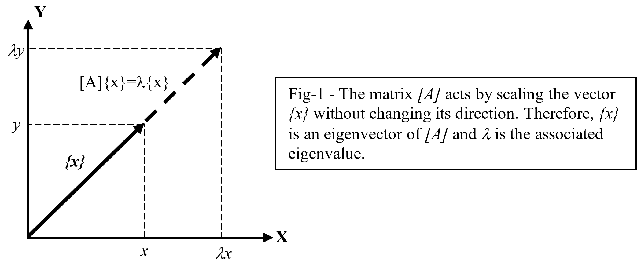
Start with ordinary matrix algebra. Let [A] be a square matrix, and let {x} be a vector. Multiplying {x} by [A] produces a new vector [A]{x}. For almost every vector you could pick, this new vector points in a different direction than the original and has a different length. Geometrically, [A] rotates and stretches most vectors.
But for a small, special set of vectors, something different happens: [A]{x} points in exactly the same direction as {x} (or the exact opposite direction). The vector is only stretched, shrunk, or flipped, never rotated off its original line. These special vectors are called eigenvectors of [A], and the scale factor that describes how much they are stretched or shrunk is called the eigenvalue.
[A]{x} = λ{x}
where [A] is a square matrix, {x} is the eigenvector, and λ (lambda) is the eigenvalue associated with that eigenvector. Rearranging this into a form you can actually solve:
[A - λI]{x} = 0
where I is the identity matrix. This single rearrangement is the hinge the entire series swings on. In Part 2, [A] becomes a mass-normalized stiffness matrix and λ becomes the square of a natural frequency. In Part 3, [A] again involves the stiffness matrix, and λ becomes a load multiplier that tells you how far you are from buckling. The physics changes completely; the algebra does not change at all.
Solving the Eigenvalue Problem by Hand
For an n-by-n matrix, solving this equation is a three-step procedure. It is worth doing by hand at least once, because every commercial FE solver (Lanczos, subspace iteration, QZ) is ultimately an efficient, large-scale way of avoiding exactly these three steps for matrices too big to handle directly.
Step 1: Form the matrix [A - λI] and compute its determinant. For an n-by-n matrix, this determinant is a polynomial in λ of degree n, called the characteristic polynomial.
Step 2: Set the characteristic polynomial to zero and solve for its roots: det[A - λI] = 0. The n roots of this polynomial are the n eigenvalues of [A].
Step 3: For each eigenvalue λ, substitute it back into [A - λI]{x} = 0 and solve for the corresponding eigenvector {x}. Because the matrix is singular at each eigenvalue by construction, this system has infinitely many solutions along one direction, which is exactly the eigenvector direction.
A Worked Numerical Example
Let’s illustrate the computation of the eigen equation with a simple two-dimensional example. Consider the following transformation matrix [A]:

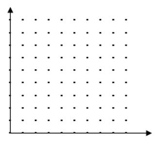
What is the effect of this transformation on the point coordinates in the following xy-plane?
The characteristic polynomial of [A] can be found by writing the determinant:

Setting this polynomial to zero will give the two roots:

λ = 1 and λ = 3 are the two eigenvalues for [A].
For λ = 1, the associated eigenvector is obtained by substituting λ = 1 in EQ 1:

The vector solving this equation is:

For λ = 3, the associated eigenvector is obtained by substituting λ = 3 in EQ 1:

The vector solving this equation is:

The vectors {v}λ=1 and {v}λ=3 are the eigenvectors of [A] associated with the eigenvalues λ = 1 and λ = 3, respectively. This result means that the transformation matrix [A] preserves the direction of vectors parallel to vectors {v}λ=1 (in purple in figure below) and {v}λ=3 (in blue in figure below). Since the red vectors are not parallel to any eigenvector, their directions are changed by the transformation. After transformation, the lengths of the blue vectors are increased by a factor of three, since their eigenvalues are 3.0, while the lengths of the purple vectors are unchanged, since their eigenvalues are 1.0.
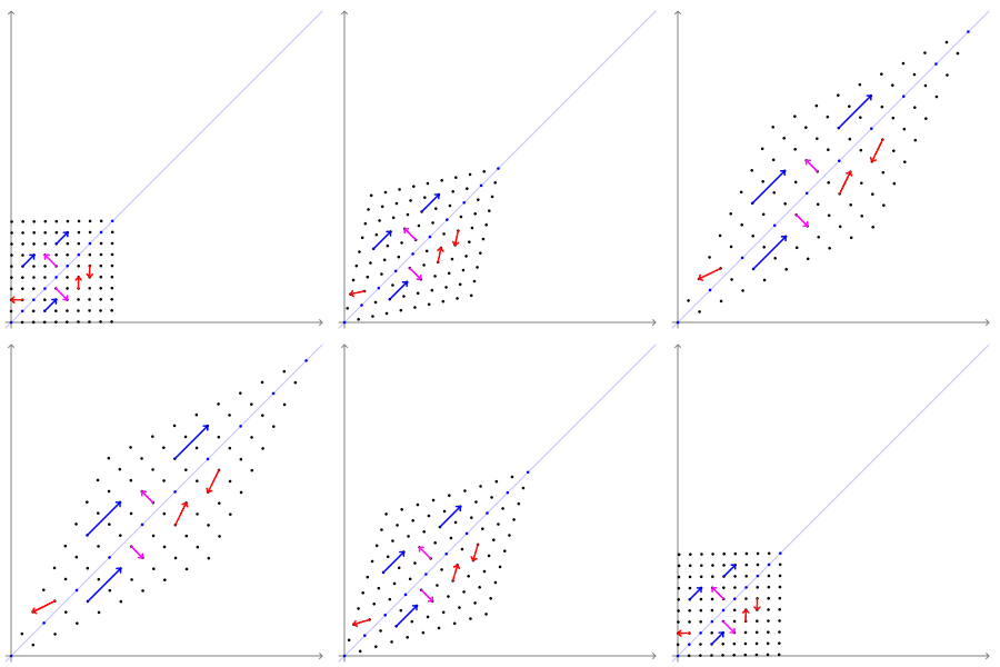
Fig-2 - Effects of the Transformation Matrix [A] on the Points Coordinates
Why the Eigenvectors Are the Useful Ones
The practical payoff is not the diagram, it is what the diagram implies about computation. If you describe a problem using an arbitrary coordinate system, like the standard x and y axes, a matrix [A] generally mixes the two coordinates together: moving in x also produces motion in y, and vice versa. But if you re-describe the exact same problem using the eigenvectors as your coordinate axes instead, that mixing disappears. Along the eigenvector directions, [A] acts like a simple number, not a matrix: it just multiplies by λ, nothing more. This is the idea of diagonalization, and it is the single reason eigenvalue problems are worth solving at all in engineering: they let you trade one coupled, n-dimensional problem for n completely independent, one-dimensional problems, each one trivial to solve on its own.
In Part 2, this is exactly what happens to the equations of motion of a vibrating structure. A structure with a thousand degrees of freedom has displacement coordinates that are all coupled to each other through the mass and stiffness matrices. Switch to mode-shape coordinates (the eigenvectors of the system) instead, and the thousand coupled equations become a thousand independent single-degree-of-freedom oscillators, each with its own natural frequency. That decoupling, and nothing else, is why modal analysis is useful rather than just mathematically interesting.
Properties Worth Knowing Before You Trust a Solver
A few structural facts about eigenvalue problems are worth internalizing now, because they explain behavior you will see in every FE eigen-solution for the rest of your career, and they set up both Part 2 and Part 3 directly.
Symmetric matrices give real eigenvalues. If [A] is symmetric (as mass and stiffness matrices always are for a physically well-posed structure), its eigenvalues are guaranteed to be real numbers, never complex. This is why a correctly formulated modal or buckling solve never hands you an imaginary natural frequency or an imaginary load factor. If you ever do see a complex eigenvalue pop out of a solver that is supposed to be solving a purely elastic, undamped problem, that is a red flag worth investigating, not a result worth reporting.
The sign of λ tells you the physical character of the mode. A positive eigenvalue corresponds to a stable, restoring behavior. A negative eigenvalue, where it is physically meaningful, corresponds to an instability. This sign test is the entire basis of a linear buckling check, covered in detail in Part 3.
Eigenvectors are only defined up to a scale factor. {v}₁ = {1, -1} and {v}₁ = {2, -2} are the same eigenvector. The direction is physically meaningful; the magnitude is arbitrary until you impose a normalization convention. FE codes resolve this ambiguity by normalizing mode shapes against the mass matrix, which is why solver output always reports a generalized (modal) mass alongside each mode.
Repeated eigenvalues are common, not exotic, in real structures. Any structure with geometric symmetry (a circular panel, a shaft, a symmetric wing box) can produce two or more eigenvalues that are identical or nearly so. When that happens, the corresponding eigenvectors are not uniquely defined individually, only the subspace they span is. It is one of the more common sources of confusion when comparing results between two solver runs or two slightly different meshes.
Practical Applications You Will Run Into This Week
Modal analysis and buckling, the subjects of Parts 2 and 3, are the two applications a structural engineer meets most often. But the same equation shows up in a few other everyday situations worth recognizing on sight.
Principal Stresses
At any point inside a loaded structure, the state of stress can be written as a 2-by-2 (plane stress) or 3-by-3 (triaxial) symmetric matrix. Most orientations of a stress element carry both normal and shear stress together. But just as in the xy-plane example above, there exist special orientations where the shear stress vanishes entirely and only normal stress remains. Those special orientations are the eigenvectors of the stress tensor, called the principal directions, and the normal stresses acting on them are the eigenvalues, called the principal stresses.
Take a plane stress state of σx = 80 MPa, σy = 20 MPa, and τxy = 30 MPa. Written as a symmetric matrix, [80 30; 30 20], its characteristic polynomial is λ² - 100λ + 700 = 0, and the same three-step procedure used above gives λ = 50 ± 42.4, that is, principal stresses of σ1 ≈ 92.4 MPa and σ2 ≈ 7.6 MPa. The eigenvector of σ1 is {30, 12.4}, which sits at 22.5 degrees from the x-axis: that is the principal direction. This is precisely why a Mohr’s circle construction works: Mohr’s circle is a graphical shortcut for an eigenvalue problem, and the two points where the circle crosses the horizontal axis are its eigenvalues. Any time you check a principal stress or a von Mises stress in a postprocessor, an eigenvalue solve already happened silently underneath, one point at a time, across the entire mesh.
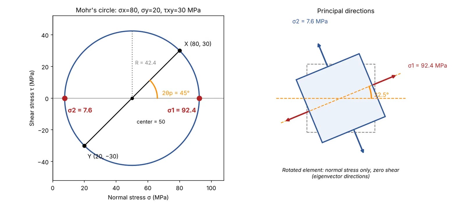
Fig-3: Mohr’s circle for the plane stress state above. The circle is centered at (σx + σy)/2 = 50 MPa with radius 42.4 MPa. Points X and Y are the stresses on the original element faces; the circle crossings on the horizontal axis are the eigenvalues. The 45 degree angle on the circle corresponds to a 22.5 degree physical rotation of the element.
Read the figure as the eigenvalue story in picture form. Point X and point Y are what the matrix shows you in the original x-y axes, with both normal and shear stress present. Rotating the element by any angle slides the stress pair around the circle at twice that angle. At the two crossings with the horizontal axis, the shear is exactly zero: those are the eigenvector directions, shown in the right panel, where only normal stress remains. Everything else on the circle is a mix of the two. The center of the circle is the average normal stress (half the trace of the matrix) and the radius is the largest shear stress the element can see, which is exactly how the eigenvalues come out as 50 ± R.
The same idea extends directly to a full 3D stress state, where the stress tensor is a 3-by-3 symmetric matrix and the eigenvalue problem produces three principal stresses, σ1 ≥ σ2 ≥ σ3, acting along three mutually perpendicular eigenvector directions, with zero shear on each of the three corresponding faces. This is also where strain, rather than stress, picks up the same machinery: the strain tensor is diagonalized the same way to find principal strains and their directions, which matters directly when you are correlating strain gauge rosette data from a test article against an FE model, since the gauge directions are almost never aligned with the principal directions the structure actually wants to report in.
Structural Optimization and Design Sensitivity
When a structural optimizer searches for a lighter design that still meets frequency or buckling margins, it is directly manipulating eigenvalues: raising the lowest natural frequency above a resonance concern, or raising the lowest buckling load factor above a required margin, often while removing mass elsewhere. Sensitivity of an eigenvalue with respect to a design variable (a skin thickness, a stringer pitch) is itself computed from the eigenvectors, because the eigenvector tells you exactly where in the structure a given mode or buckling shape is storing its energy, and therefore where a design change will move the needle most. A stiffener added where a mode shape shows large displacement moves that mode’s frequency a lot; the same stiffener added where the mode shape is near zero barely moves it at all, no matter how much material you add. Reading the eigenvector before you resize anything is what separates an efficient optimization iteration from a lucky one.
A Word on Complex Eigenvalues: Stability and Flutter
Everything above assumes [A] is symmetric, which guarantees real eigenvalues. Once damping or aerodynamic coupling enters the picture, as it does in a flutter stability analysis, the governing matrix is no longer symmetric, and the eigenvalues can become complex: λ = α + iβ. The physical reading of a complex eigenvalue is direct and important to know even outside the detailed flutter math. The imaginary part, β, gives an oscillation frequency, exactly as before. The real part, α, now tells you whether that oscillation grows or decays with time: a negative real part means the oscillation dies out (a stable, damped mode), and a positive real part means the oscillation grows without bound (an instability). This is precisely the mechanism behind flutter: as airspeed increases, aerodynamic forces progressively couple two or more structural modes together, and at the flutter speed, the real part of one eigenvalue crosses from negative to positive. The structure does not fail because a load exceeds a strength, it fails because an eigenvalue crosses zero. This is outside the scope of this series, but it is worth knowing that the same family of equation introduced here is the one flutter analysts are watching move across the complex plane.
How Large FE Models Actually Solve This
The three-step hand procedure above does not scale. A real aircraft structure FE model can have hundreds of thousands to tens of millions of degrees of freedom, and forming an explicit characteristic polynomial of that degree is neither possible nor necessary, since you almost never need all of the eigenvalues, only the lowest handful. Production solvers instead use iterative, sparsity-preserving methods: the Lanczos algorithm (the most common choice in codes like Nastran’s SOL 103 and SOL 105) builds up a small Krylov subspace that captures the lowest modes without ever forming the full matrix inverse, and subspace iteration methods achieve something similar through repeated matrix-vector products. Shift-and-invert strategies let you target a specific frequency or load band away from zero, which is how you extract, say, only the modes between 20 and 200 Hz instead of starting from zero every time. None of this changes the underlying equation; it only changes how efficiently you get to the same answer Step 1 through Step 3 would eventually give you by hand.
Common Pitfalls When Reading Eigenvalue Output
A handful of practical issues account for most of the confusion engineers run into when looking at modal or buckling solver output. Recognizing them here saves real debugging time later in Parts 2 and 3.
Missing modes because the extraction range was too narrow. Most solvers only search for eigenvalues inside a frequency or load band you specify. A mode sitting just outside that band is silently absent from the output, not flagged as missing, so always extract a few more modes than you think you need and check the band edges.
Eigenvector sign flips between runs. Because {v} and -{v} are the same eigenvector, a solver is free to return either sign, and a small mesh or solver-version change can flip it. Do not read a sign flip between two runs as a change in physical behavior.
Unconstrained models showing near-zero eigenvalues. A free-free structure (no boundary conditions applied, common when checking a model before it is installed in an assembly) should show exactly six near-zero frequency modes in 3D, corresponding to the six rigid body motions. This is one of the most useful FE model sanity checks available: if you see five or seven near-zero modes instead of six, something is wrong with your connectivity or mass distribution before you ever get to the flexible modes that matter.
Closely spaced or repeated eigenvalues changing shape between mesh refinements. As flagged above, when two eigenvalues are nearly equal, their eigenvectors are not individually unique, only the subspace they span is. A slightly different mesh or solver can mix the two mode shapes together in a different proportion while leaving the physics, and the frequencies, essentially unchanged. This is normal behavior for symmetric or near-symmetric structures, not a modeling error.
What Comes Next
Continuing the series
Part 2 of this series takes the exact equation [A - λI]{x} = 0 developed here and applies it to a system in free vibration, an avionics box mounted on an isolator bracket. You will see the generalized eigenvalue problem [K]{φ} = ω²[M]{φ} derived from first principles, solved by hand, and interpreted mode by mode, with a direct tie to how you read a modal results table coming out of a solver like Nastran.
Part 3 then shows that the same framework, with the stiffness matrix paired against a geometric stiffness matrix instead of the mass matrix, predicts the load at which a structure buckles, worked through a landing gear drag strut example with a direct link to certification margin.