



In this series
This is Part 2 of a three-part series on eigenvalues and eigenvectors for practicing structural and FEA engineers. Part 1: The Mathematical Foundation introduced the equation [A]{x} = λ{x}, showed how to solve it by hand on a simple 2-by-2 matrix, and previewed where it shows up across structural engineering. If any of that is unfamiliar, it is worth reading first.
This article takes that exact equation and applies it to a real engineering problem: predicting how an aerospace structure vibrates on its own, with no external forcing. Part 3: How the Same Eigenvalue Problem Predicts Structural Instability then shows that the same framework, with one matrix swapped out, predicts buckling instead.
A note before you start reading
This article is deliberately hands-on. It contains a lot of equations and numerical applications, worked step by step so that you can follow every line with a calculator.
I have verified all of my calculations, but with this many numbers, an error may still have slipped through. If you find one, I would welcome your message: please contact me through fea-academy.com or send me a direct message on LinkedIn, and I will update the article. Thank you.
A Real Failure to Start With
In 1959 and 1960, three Lockheed Electra turboprop airliners suffered in-flight wing separations. The investigation traced the cause to a phenomenon called whirl-mode flutter: a propeller and gearbox assembly, given a slightly weakened engine mount, could precess (whirl) at a frequency that fell close enough to the wing’s own bending and torsion natural frequencies to couple with them. Once coupled, the combined system no longer damped itself out; it fed energy into the oscillation instead of dissipating it, and the amplitude grew until the wing failed. The fix was a stiffer engine mount, which pushed the whirl frequency safely away from the wing’s structural frequencies.
Strip away the aerodynamics and the failure mechanism, and the engineering question underneath the Electra accident is the same question underneath every modal analysis you will ever run: what frequencies does this structure naturally want to vibrate at, and in what shape? Get that answer wrong, or get a structural change that moves a frequency into a dangerous band without anyone noticing, and the consequences can be exactly this severe. Get it right, and you have a frequency map you can use to keep every rotating, pulsing, or gusting input your structure will see safely away from a resonance.

From the Equation of Motion to an Eigenvalue Problem
Consider a structure idealized, as every FE model is, as a set of discrete mass points connected by elastic stiffness. For free vibration, with no external force and no damping, Newton’s second law applied to every degree of freedom at once gives the matrix equation of motion:
[M]{ü} + [K]{u} = {0}
where [M] is the mass matrix, [K] is the stiffness matrix, and {u} is the displacement vector, with the double dot denoting acceleration. This is a system of coupled second-order differential equations: every mass is connected to its neighbors through [K], so you cannot, in general, solve for one degree of freedom’s motion without knowing all the others at the same time.
Now make the harmonic assumption that is the entire basis of modal analysis: assume the structure can vibrate in a fixed spatial shape, {φ}, that simply grows and shrinks sinusoidally in time, with every point moving in or out of phase together and no point’s shape relative to the others ever changing.
{u(t)} = {φ} sin(ωt)
Substituting this assumed form into the equation of motion and dividing through by sin(ωt) gives:
([K] - ω²[M]){φ} = {0}
Compare this directly to Part 1’s equation, [A - λI]{x} = 0. The structure is identical, with [M] standing in for the identity matrix and ω² standing in for λ. This is called a generalized eigenvalue problem, and it is the governing equation of every modal analysis ever run:
[K]{φ} = ω²[M]{φ}
The eigenvalues ω² are the squares of the structure’s natural circular frequencies; the eigenvectors {φ} are its mode shapes. As in Part 1, a nontrivial solution exists only where [K - ω²M] is singular, giving the characteristic equation det[K - ω²M] = 0, whose n roots are the n natural frequencies of an n-degree-of-freedom model.
It is worth pausing on why the harmonic assumption is reasonable before trusting the algebra that follows from it. A linear, undamped structure has no mechanism to change a motion’s shape once it is set in motion: energy sloshes back and forth between kinetic energy and strain energy, but nothing in the equation of motion favors one spatial pattern over another or redistributes energy between unrelated patterns. Assuming the structure holds a fixed shape while oscillating is therefore not an approximation imposed on the physics, it is the one assumption consistent with a linear, time-invariant system, and solving for which shapes actually satisfy it is exactly the eigenvalue problem that follows.
A Worked Example: Isolating an Avionics Box
Vibration isolation is one of the places a structures engineer meets this equation most directly, because the design intent (keep a sensitive box away from the airframe’s vibration environment) lives or dies on getting the natural frequencies right. We will solve one small case completely by hand, step by step, with every intermediate number shown, so that you can check each line on a calculator. It is the same procedure an FE solver runs, just on two degrees of freedom instead of two million.
Step 1: Define the model and the data
An avionics box is mounted on elastomer isolators. The isolators sit on a small equipment bracket, and the bracket is bolted to the airframe. We idealize this as two lumped masses connected by two springs, as shown in Fig. 1. The airframe is treated as fixed (it is far heavier and stiffer than the bracket), and each mass moves only vertically, so the model has two degrees of freedom: u₁, the box displacement, and u₂, the bracket displacement. Both are measured from the static equilibrium position, positive upward. Gravity only shifts that equilibrium position, so it drops out of the vibration problem.
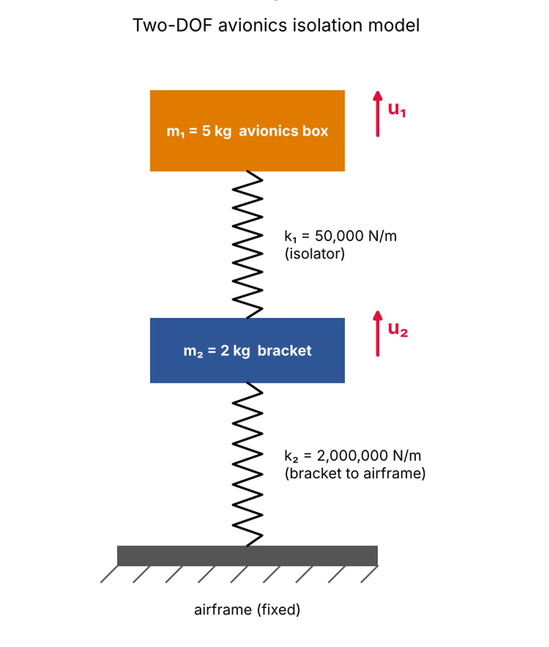
Fig. 1: Two-DOF model. The soft isolator k₁ links the box to the bracket; the stiff attachment k₂ links the bracket to the airframe.

Work in consistent SI base units: kilograms, newtons per meter, seconds. The eigenvalues then come out directly in (rad/s)². Mixing N/mm stiffness with kg mass, or tons with N/mm without checking, is the most common reason a hand check and an FE result disagree by a factor of 1,000 or of √1,000 ≈ 31.6.
Step 2: Write the equations of motion
Draw a free body diagram of each mass. The isolator spring is stretched by the relative displacement (u1 − u2); it pulls the box back down with a force k1(u1 − u2) and pulls the bracket up with the same force. The attachment spring is stretched by u2 alone, since the airframe does not move, and pulls the bracket down with a force k2u2. Newton’s second law for each mass gives:
m1ü1 = −k1(u1 − u2)
m2ü2 = +k1(u1 − u2) − k2u2
Moving every term to the left-hand side and grouping by displacement:
m1ü1 + k1u1 − k1u2 = 0
m2ü2 − k1u1 + (k1 + k2)u2 = 0
The two equations are coupled: u2 appears in the box equation and u1 appears in the bracket equation. Neither mass can be solved for on its own, which is exactly the situation modal analysis is designed to resolve.
Step 3: Assemble the mass and stiffness matrices
Writing the two equations in matrix form [M]{ü} + [K]{u} = {0} gives:

Each stiffness term has a direct physical reading: Kij is the force needed at degree of freedom i to hold a unit displacement at degree of freedom j, with every other degree of freedom held at zero. Push the box up by 1 m with the bracket held still and the isolator resists with k1 on the box and −k1 on the bracket: that is column 1. Push the bracket up by 1 m with the box held still and both springs react on the bracket, giving k1 + k2, while the isolator pulls on the box with −k1: that is column 2. Three properties are worth checking on any matrix you assemble, by hand or in an FE code:
• [K] is symmetric (K12 = K21 = −50,000 N/m), as Maxwell’s reciprocity theorem requires.
• [M] is diagonal because the masses are lumped at points with no inertial coupling between them.
• Every diagonal term is positive and the structure is restrained, so both matrices are positive definite. As shown in Part 1, this guarantees real, positive eigenvalues.
Step 4: Form the eigenvalue problem and its characteristic equation
Substituting the harmonic solution {u} = {φ} sin(ωt) gives ([K] − ω2[M]){φ} = {0}. To keep the algebra readable, write x = ω2. Subtracting x times [M] from [K] term by term:

A nonzero mode shape exists only if this matrix is singular, so its determinant must vanish. For a 2-by-2 matrix, the determinant is the product of the diagonal terms minus the product of the off-diagonal terms:
(50,000 − 5x)(2,050,000 − 2x) − (−50,000)(−50,000) = 0
Expanding term by term, collecting then dividing through by 10:
10x2 − 10,350,000x + 100,000,000,000 = 0
x2 − 1,035,000x + 10,000,000,000 = 0
It is worth writing the same equation symbolically once, because it shows where each coefficient comes from and gives two free checks on the arithmetic:
m1m2x2 − [m2k1 + m1(k1 + k2)]x + k1k2 = 0
For any quadratic, the sum of the roots equals minus the middle coefficient divided by the leading one, and the product equals the constant divided by the leading one. Here, ω12 + ω22 must equal 1,035,000 and ω12·ω22 must equal k1k2/(m1m2) = 1010. We will use both checks in a moment.
Step 5: Solve for the natural frequencies
Apply the quadratic formula:
x = [1,035,000 ± √(1,035,0002 − 4 × 10¹⁰)] / 2
√(1,071,225,000,000 − 40,000,000,000) = √(1,031,225,000,000) = 1,015,492.5
x1 = (1,035,000 − 1,015,492.5) / 2 = 9,753.8 (rad/s)2
x2 = (1,035,000 + 1,015,492.5) / 2 = 1,025,246 (rad/s)2
Check: 9,753.8 + 1,025,246 = 1,035,000 and 9,753.8 × 1,025,246 = 1.000 × 10¹⁰. Both checks pass. Taking the square root gives the circular frequency ω in rad/s, and dividing by 2π gives the frequency f in hertz:

Before going further, run the sanity check every experienced structural dynamicist does reflexively: estimate each frequency as if the other mass were not there. The box alone on its isolator, with a rigid bracket underneath, would vibrate at √(k1/m1) = √(50,000/5) = 100 rad/s, or 15.9 Hz. The bracket alone, held by both springs with the box held still, would vibrate at √((k1 + k2)/m2) = √(2,050,000/2) = 1,012.4 rad/s, or 161.1 Hz. The coupled answers, 15.72 Hz and 161.15 Hz, sit right next to these estimates. That tells you the two masses barely interact. It also shows a general rule: coupling always pushes the two frequencies slightly apart, so the lower mode drops a little (15.9 to 15.72 Hz) and the upper one rises a little (161.1 to 161.15 Hz).
Step 6: Solve for the mode shapes
Exactly as in Part 1’s Step 3, substitute each eigenvalue back into ([K] − x[M]){φ} = {0}. Because the matrix is singular at each root, its two rows are proportional and carry the same information, so one row is enough. The first row reads:
(50,000 − 5x)φ1 − 50,000φ2 = 0 → φ1/φ2 = 50,000 / (50,000 − 5x)
Only the ratio φ1/φ2 is determined, never the absolute values. That is the scale ambiguity from Part 1, so we are free to set the bracket amplitude φ2 = 1.
Mode 1 (x1 = 9,753.8 (rad/s)2):
50,000 − 5 × 9,753.8 = 50,000 − 48,768.8 = 1,231.2
φ1/φ2 = 50,000 / 1,231.2 = 40.61 → {φ}1 = {40.61, 1}T
Check with the second row: −50,000 × 40.61 + (2,050,000 − 2 × 9,753.8) × 1 = −2,030,500 + 2,030,492 ≈ 0. The small residual is rounding in 40.61. The row checks out.
Mode 2 (x2 = 1,025,246 (rad/s)2):
50,000 − 5 × 1,025,246 = 50,000 − 5,126,230 = −5,076,230
φ1/φ2 = 50,000 / (−5,076,230) = −0.00985 → {φ}2 = {−0.00985, 1}T
Read the signs and the ratios, because they are the whole physical story:
• Mode 1, 15.7 Hz, the isolator mode. Both entries are positive, so box and bracket move in phase. The box moves 40.6 times more than the bracket; put differently, the bracket moves only 1/40.6 = 2.5% of the box amplitude. The box is bouncing on its soft isolator while the stiff bracket underneath barely moves.
• Mode 2, 161.2 Hz, the bracket mode. The entries have opposite signs, so box and bracket move out of phase. The box moves only 0.985% of the bracket amplitude. The bracket is vibrating on its stiff attachment while the box, hanging on the soft isolator, stays almost still.
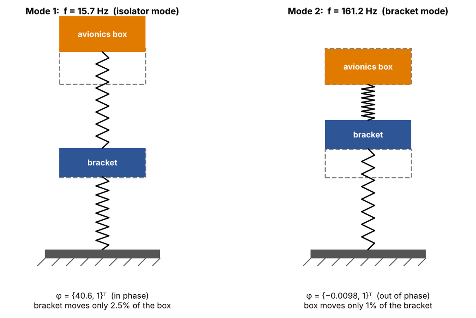
Fig. 2: The two mode shapes. Mode 1 is dominated by the box on its isolator; Mode 2 is dominated by the bracket, with the box nearly stationary.
Step 7: Verify orthogonality and normalize the modes
Two quick calculations confirm the result and connect it to what an FE solver prints. First, orthogonality with respect to the mass matrix, {φ}1T[M]{φ}2 = 0. Because [M] is diagonal, this reduces to a mass-weighted dot product of the two shapes:

The two modes are mass-orthogonal, as the theory requires. The same check with [K] also returns zero, to rounding. Second, the generalized (modal) mass and stiffness of each mode. To avoid confusing them with the box mass m1 and isolator stiffness k1, we write them Mgen,i = {φ}iT[M]{φ}i and Kgen,i = {φ}iT[K]{φ}i:
Mgen,1 = 5(40.61)2 + 2(1)2 = 8,247.8 kg
Kgen,1 = Mgen,1ω12 = 8,247.8 × 9,753.8 = 80.45 × 10⁶ N/m
Mgen,2 = 5(−0.00985)2 + 2(1)2 = 2.0005 kg
Kgen,2 = Mgen,2ω22 = 2.0005 × 1,025,246 = 2.051×10⁶ N/m
A modal mass of 8,247.8 kg for a 7 kg system looks alarming, but it means nothing physically. It simply reflects the arbitrary choice φ2 = 1, which made the box entry 40.61. This is why FE codes mass-normalize: each mode shape is divided by √(Mgen,i) so that its generalized mass becomes exactly 1. Dividing by √8,247.8 = 90.82 and by √2.0005 = 1.4144:

After mass normalization, each mode’s modal stiffness equals its eigenvalue ωi2, which is exactly what the last column shows. The mass-normalized shapes are what you would find in a MSC NASTRAN SOL103 (Modal Analysis) output with the default normalization (units of 1/√kg), and the generalized mass column would read 1.0 for every mode. If you ever compare a hand calculation with solver output and the shapes look different, check the normalization before you check anything else.
Step 8: Translate the numbers into design decisions
The eigenvalue solution is only useful once it answers the design question: does the isolator protect the box? For a single-degree-of-freedom isolator, a classical result is that vibration is attenuated only at frequencies above √2 times the isolator natural frequency; below that, the isolator amplifies, and near the natural frequency it amplifies strongly. With f1 = 15.72 Hz, isolation starts at √2 × 15.72 ≈ 22.2 Hz. Three practical conclusions follow:
• Above about 22 Hz, the box is protected, and the protection improves as frequency increases. Most propeller, rotor, engine and aerodynamic content in the tens to hundreds of hertz falls in this zone.
• Any airframe input near 15.7 Hz is a problem. A blade-pass or shaft harmonic, or a low airframe mode, at or near that frequency would be amplified at the box instead of attenuated. The first check on any isolator design is a list of forcing frequencies compared against f1; a common rule of thumb keeps f1 at least a factor of 2 to 3 below the lowest significant forcing frequency.
• The bracket resonance at 161 Hz barely reaches the box. In Mode 2 the box moves less than 1% of the bracket amplitude. The bracket still needs its own fatigue and strength check at that frequency, but the isolator decouples the box from it. This is the payoff of the factor of 10 separation between f1 and f2.
If a design change ever raised k1 enough to push f1 toward f2, the two modes would start to share motion, the clean 40:1 and 1:100 amplitude ratios above would blur, and the isolator would stop doing its job. It is the same coupling mechanism, in miniature and without the aerodynamics, that brought down the Electra’s wing.
Orthogonality: Why This Decouples at All
Because [M] and [K] are both symmetric, the mode shapes satisfy a property called orthogonality with respect to both matrices:
{φ}ᵢᵀ[M]{φ}ⱼ = 0
and
{φ}ᵢᵀ[K]{φ}ⱼ = 0 for i ≠ j
Physically, this says that distinct modes do not exchange energy with each other: kinetic energy associated with one mode’s motion, projected through the mass matrix onto another mode, vanishes exactly. This is precisely the diagonalization idea introduced in Part 1: describing the structure’s motion in mode-shape coordinates instead of physical displacement coordinates turns the coupled two-equation system above into two completely independent single-degree-of-freedom oscillators, one at 15.72 Hz and one at 161.15 Hz, each solvable on its own.
For the diagonal (i = j) terms, define the modal mass and modal stiffness of each mode:
Mgen,i = {φ}iT[M]{φ}i Kgen,i = {φ}iT[K]{φ}i ωi2 = Kgen,i/Mgen,i
Recall from Part 1 that eigenvectors are only defined up to an arbitrary scale factor; the shape {40.61, 1} and the shape {4.061, 0.1} describe exactly the same mode, as Step 7 above showed. FE solvers resolve this ambiguity with mass normalization, scaling each mode shape so that M_gen,i = 1, which then makes K_gen,i equal to ωᵢ² directly. This is why a modal results table from a solver like Nastran’s SOL 103 always reports a generalized mass column alongside each frequency: it is telling you how the raw mode shape output was scaled, which matters the moment you try to use that mode shape for anything quantitative downstream, such as a forced response or a random vibration analysis.
Reading a Modal Results Table Like an Engineer
A production modal solve on a model with a few hundred thousand degrees of freedom will typically report, for each extracted mode: a mode number, a natural frequency, a generalized (modal) mass, and an effective mass fraction in each of the six global directions.
The effective mass fraction is the practical, everyday use of orthogonality: it tells you, for a given mode, what fraction of the total structural mass that mode is capable of moving if excited in a given direction.
A mode with a tiny effective mass fraction in the direction you care about will barely respond to a load applied in that direction, no matter how perfectly tuned its frequency is to the input, and can usually be left out of a forced-response or random vibration analysis without materially affecting the result.
This is the standard, defensible way to decide how many modes to keep in a dynamic analysis without exhaustively running every single one: extract modes up to some frequency comfortably above your highest excitation frequency of interest, sum the effective mass fractions in each direction, and confirm the running total captures on the order of 80 to 90 percent or more of the total mass in that direction. If it does not, the truncated mode set is missing a mode that matters, usually a stiff, high-frequency local mode that nonetheless carries significant mass, and extending the frequency range of the extraction, not adding arbitrary extra modes, is the fix.
The Free-Free Rigid Body Check
One of the single most useful, and most underused, modeling checks available to a structures engineer comes directly out of this same equation. Run a modal analysis on a structure with no boundary conditions applied at all, a free-free model, and the stiffness matrix [K] is only positive semi-definite rather than positive definite: there exist whole-structure motions, the six rigid body translations and rotations, that produce zero strain energy and therefore zero restoring force.
Solving [K]{φ} = ω²[M]{φ} on such a model should return exactly six eigenvalues at, or numerically indistinguishable from, zero, with mode shapes that are pure rigid body translations and rotations, before the first flexible mode appears. This is a near-universal first check run on a new or heavily modified FE model before trusting anything else out of it: six clean, near-zero modes confirm the mass matrix, element connectivity, and material property definitions are at least consistent with each other. Five modes, seven modes, or six modes that are not numerically close to zero, is a direct, early signal that something in the model, commonly a disconnected element, a missing mass property, or an unintended constraint, needs fixing before the flexible modes above it can be trusted at all.
Sensitivity: What Happens If the Isolator Gets Stiffer
It is worth pushing the worked example one step further, because the eigenvalue sensitivity it reveals is exactly the kind of judgment a frequency analysis is supposed to build.
Suppose a later design change, perhaps a tighter fastener torque specification or a stiffer elastomer compound, raises the isolator stiffness from k₁ = 50,000 N/m to k₁ = 400,000 N/m, with everything else unchanged. Re-solving the same 2-by-2 eigenvalue problem pushes the first mode from 15.7 Hz up to roughly 40.9 Hz, while the second mode moves only modestly in comparison, from 161.2 Hz to about 175.3 Hz.
The isolator mode is sensitive to k₁ because its eigenvector puts almost all the displacement into m₁, exactly where k₁ acts; the structural mode is insensitive to k₁ because its eigenvector puts almost all the displacement into m₂, where k₁ barely participates.
This is the general rule from Part 1 in action: an eigenvalue only moves significantly when a design change acts where the corresponding eigenvector already shows motion, and a stiffness or mass change placed where a given mode shape is near zero will not move that mode’s frequency no matter how large the change is.
Reading the eigenvector before deciding where to stiffen a structure is what turns this from guesswork into a one-pass design decision.
Pitfall: Confusing Local Modes With Global Modes
Ordering modes strictly by ascending frequency, which every solver does by default, quietly assumes that frequency order lines up with some intuitive hierarchy of importance, global modes first, then progressively more local detail. Real structures do not cooperate with that assumption.
A thin access panel, a lightly supported bracket, or a long unsupported cable bundle can produce a low-frequency local mode that falls numerically below, or interleaved with, the global wing or fuselage bending modes an analyst actually came looking for. Skimming a modal results table by frequency alone, without checking each mode’s effective mass fraction and glancing at its shape, is a common way to either miss the global mode you actually care about or spend review time chasing a local panel mode that carries almost no mass and will not meaningfully respond to any realistic excitation.
The effective mass fraction introduced above is exactly the filter that separates the two cases quickly.
Ground Vibration Testing: Closing the Loop With Reality
An FE-predicted mode set is a prediction, not a measurement, and for any structure where getting the frequencies right actually matters, such as an aircraft that will later be cleared for flutter across its speed envelope, that prediction gets checked against a ground vibration test (GVT) before it is trusted. A GVT instruments the real structure with accelerometers, excites it with shakers or an instrumented hammer across a frequency sweep, and extracts measured natural frequencies and mode shapes using the same underlying eigenvalue mathematics applied to the measured response instead of to [M] and [K] directly.
The standard way to compare a measured mode shape against its FE-predicted counterpart is the Modal Assurance Criterion (MAC), a normalized dot product between the two eigenvectors that returns 1.0 for a perfect shape match and drops toward zero as the shapes diverge, independent of amplitude or sign, which is convenient given that eigenvectors are only defined up to an arbitrary scale and sign in the first place, exactly as established in Part 1.
A high MAC value paired with a frequency that is off by a few percent usually points to a mass or stiffness value that needs correcting in the model; a low MAC value, even with a close frequency match, is a more serious warning that the FE model and the test article are not vibrating in the same shape at all, and two unrelated modes have simply landed close together in frequency by coincidence.
Model updating, the process of adjusting boundary conditions, joint stiffnesses, or nonstructural mass in the FE model until both frequency and MAC line up with test data, is the standard closing step before an FE model is cleared to support certification work such as a flutter analysis.
From Modes to Forced Response
Modal analysis on its own, as presented above, only answers how a structure vibrates with nothing pushing on it. The practical payoff comes from modal superposition: because the mode shapes form a complete, orthogonal basis, any physical response of the structure, under any time-varying or frequency-varying load, can be expressed as a combination of its mode shapes, each one responding as an independent single-degree-of-freedom oscillator to the portion of the load that projects onto it (its modal participation factor). This is how a transient landing load, a random vibration spectrum from a test specification, or a sine sweep from a qualification test all get analyzed efficiently on models far too large to integrate directly in physical coordinates: solve the eigenvalue problem once, then reuse the same handful of decoupled modal equations for every load case that follows.
Damping complicates this picture slightly, since a general damping matrix does not share the mass and stiffness matrices’ orthogonality and can reintroduce coupling between modes. The common engineering workaround, proportional (Rayleigh) damping, defines [C] = α[M] + β[K] specifically so that the same mode shapes remain orthogonal with respect to [C] as well, letting each decoupled modal equation carry its own modal damping ratio, ζᵢ, without disturbing the clean structure derived above. This is why proportional damping is the default assumption in the overwhelming majority of production dynamic analyses, even though it is a simplification of how real structures actually dissipate energy.
What Comes Next
Continuing the series
The generalized eigenvalue problem in this article, [K]{φ} = ω²[M]{φ}, paired the stiffness matrix against the mass matrix. Part 3: How the Same Eigenvalue Problem Predicts Structural Instability pairs the stiffness matrix against a different matrix instead, the geometric stiffness matrix built from an applied load, and shows that the resulting eigenvalues are load multipliers rather than frequencies: the same algebra, a different physical question entirely. It is worked through a landing gear drag strut example, closed-form Euler buckling check included, with a direct link to how a buckling eigenvalue becomes a certification margin.
Go Further: Modal Analysis in Practice
If you would like to go further and see how modal analysis by FEA is applied in an industrial context, I invite you to watch my dedicated YouTube video: FEA Insight, Ep. #12: Introduction to Modal Analysis by FEA.